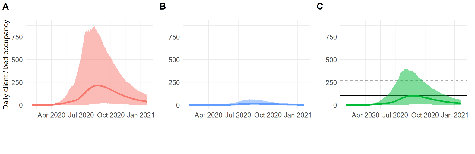
 Excerpt from our working paper. Figure shows planning simulations for A) Home health care counts, B) Hospice care counts, and C) Skilled nursing facility counts based on a specific policy scenario. THIS IS NOT A FORECAST; it’s a scenario-based projection used for planning purposes, based on data available at the time of the publication of the working paper.
Using Bayesian Statistics to Plan for COVID-19 Post-Acute Care
A Collaboration with Researchers and Clinicians at University of Utah Health
Background
Uncertainty has been defining our personal and professional lives since the early March, when COVID-19 began spreading widely in the United States. Predictive modeling, as used for forecasting and policy analysis, has become a central tool for managing this uncertainty. The Johns Hopkins University Infectious Disease Dynamics (JHU IDD) model is one of the most advanced models that has been developed to date. It has been widely used to assist COVID-19 planning efforts and the open-source code can be found here. Thanks to Lindsay Keegan, PhD, an assistant professor in the University of Utah School of Medicine Division of Epidemiology, this model has been one of the tools used by the State of Utah and University of Utah Health System to manage and plan for COVID-19.
Dr. Keegan is an infectious disease modeling expert who was previously a Postdoctoral Fellow at the Johns Hopkins Bloomberg School of Public Health. She has led the effort to adapt and deploy the JHU IDD model to aid the University of Utah and State of Utah in COVID-19 planning and policy analysis, and I recently had the privilege of working with her on an extension of the JHU IDD model. My typical focus at University of Utah Health (U Health) is the application of data science and research methods to further long-term planning, strategy, and operational objectives. However, it has been all hands on deck for the COVID-19 response, and I was recruited by Dr. Keegan and U Health’s Population Health group to assist with planning for U Health and the State of Utah’s COVID-19 related post-acute care needs. Specifically, they needed a way to extend the planning simulations from the JHU IDD model (e.g., cases, hospitalizations, ICU bed requirements, etc.) to include post-acute care outcomes (e.g., the number of COVID-19 patients who will require a skilled nursing facility, a home health aid, etc.). I was selected to lead the modeling efforts with the help of Robert Checketts from U Health’s data engineering team.
This post is an informal overview of the project that includes commentary on some aspects of the project I found interesting. For more detail, see our working paper or the project’s code repository.
An opportunity for Bayesian thinking
This was a perfect application for Bayesian statistics. At the time the project started, I had no data on COVID-19 post-acute care outcomes. Not a single observation. But I did have access to subject matter experts with well-informed priors about the approximate percentage of discharged patients who will require each type of post-acute care service. We also needed an approach that would allow us to update these priors over time as we observed the post-acute care needs of actual COVID-19 discharges from the University of Utah Hospital.
The desired product was code that could take the output from the JHU IDD model, in the form of thousands of simulations of hospitalizations and discharges, and allocate each discharge to one of four post-acute care outcomes:
- None: the discharged patient goes directly home without any additional care needs
- Home Health (HH): the discharged patient requires a home health aid
- Skilled Nursing Facility (SNF)
- Hospice Care (HOS)
I won’t go into detail about Bayesian vs Frequentist statistics in this post (there are plenty of good resources with varying degrees of technical detail), but this way of framing the problem is rooted in Bayesian thinking. Bayesian statistics allows us to (1) talk about the problem in a way that is consistent with how everyone is thinking about the problem anyway: we have some subjective idea about the percentage of patients who will need each type of post-acute care service, but we don’t know precisely, and (2) we don’t have to wait to collect data to begin making predictions about post-acute care needs, and can seamlessly incorporate new data as it becomes available.
I needed to very quickly develop code to add to the modeling pipeline that Dr. Keegan was running every couple of weeks to provide planning reports to health system and state leadership. So, not a lot of time for developing a complex model. Relative simplicity was essential. I knew that we needed to (1) formalize our uncertainty into a prior distribution and (2) set up a system for updating those priors as new data became available.
Formalizing the uncertainty with a probabilistic model
The JHU IDD model generates thousands of separate simulations for various planning scenarios to produce a range of possible outcomes conditional on specific policy choices. An output of these simulations is a series of discharge counts. To extend these simulations to also predict post-acute care needs, the simplest solution would have been to choose some fixed parameters for a multinomial distribution and then draw from this distribution to allocate total discharge counts to post-acute care (PAC) outcomes (none, home health, skilled nursing facility, or hospice care). The multinomial distribution has
| Parameter | Definition |
|---|---|
| n | number of discharges |
| pnone | probability of not requiring any PAC service |
| phh | probability of requiring home health aid |
| psnf | probability of requiring a skilled nursing facility (SNF) |
| phos | probability of requiring hospice care (HOS) |
This very simple approach fails to account for our uncertainty – what should correct probabilities/parameters be? This was the core problem that I actually needed to solve. Given our uncertainty, what is the worst case scenario for post-acute care needs? The best case scenario?
The Dirichlet distribution allows us to formalize this uncertainty. Each random draw from a Dirichlet distribution produces
Creating the prior distributions
For formulating priors, I had at access to two subject matter experts (SMEs) from the University of Utah: Dr. Peter Weir, the Executive Medical Director of Population Health, and Ryan Morley, the Director of Population Health. I started our engagement by getting their rough estimates of what the probabilities of a COVID-19 patient needing each of the four post-acute categories might be after being discharged. I asked them for two sets of probabilities: one set for patients who spent time in the Intensive Care Unit (ICU) and one for patients who did not, as this single fact provides an enormous amount of information about the seriousness of their condition and the likelihood of requiring PAC services. In other words, we decided to condition the probabilities on ICU status. Table 2 shows their initial best estimates:
| Parameter | SME ICU Estimate | SME Non-ICU Estimate |
|---|---|---|
| pnone | 0.49 | 0.75 |
| phh | 0.20 | 0.18 |
| psnf | 0.30 | 0.06 |
| phos | 0.01 | 0.01 |
As a starting point, I got their best estimates for the probability of a discharged COVID-19 patient requiring one of the four PAC services (none, HH, SNF, or HOS). This resulted in two sets of four parameters (one set for ICU patients and one set for non-ICU patients). To translate these into a parameter set we could use for the Dirichlet distribution, I needed to multiply these by a weight that quantifies the confidence we had regarding how close these were to the truth. This weight, which I will call
The Dirichlet distribution can be visualized precisely when it has three parameters (e.g., link), but visualizing when there are four or more it can be tricky (in this case, there are four). One approach is to plot the distributions of the individual outputs. This visualization falls short in that one is not able to see the dependence between individual draws (all of the output values from a single draw must equal one), but it gives one a general idea of the range of observable values for each output. I created an interactive version of this visualization below. Changing the ‘Prior Weight’ will alter how concentrated values will be around the initial estimates for
I worked with Dr. Weir and Mr. Morley to determine the proper weight for the prior distribution. I asked them to provide a range of values they thought plausible, and showed them a similar visualization as the one above to help further hone our intuition about the appropriate prior distribution. This process led us to choose weights of 138 for the ICU discharges and 121 for non-ICU discharges.
Next, Robert Checketts and I divided the programming tasks and built a module that could be run as an add-on to the JHU IDD pipeline. We are now able to run new PAC simulations every couple of weeks as Dr. Keegan runs more JHU IDD simulations.
Updating the prior distributions
Every time we run new PAC simulations, we first update the Dirichlet prior distribution based on the COVID-19 discharges we observed since the last run. The Dirichlet prior and posterior distributions are conjugate distributions and updating the prior with new information is very easy – all one has to do is take the observed counts and add them to the Dirichlet parameters. That is, one only has to add the observed counts to the ‘pseudo counts’ from the prior. This updating process has the effect of shifting the mean values towards their ‘true’ values and tightening the range of each value that is drawn from the Dirichlet. This, in turn, reduces the prediction intervals in our simulations of future post-acute care service needs. Figure 1 shows how our expectations about the percentage of patients who will require each PAC service have changed over time as we have observed discharges from the University of Utah Hospital.
Figure 1: Incorporating new information over time. The x-axis shows days since we began tracking discharge data. The left-side plots compare the cumulative observed fraction of University of Utah COVID-19 patients discharged to each care service with our initial expectations for Non-ICU (A) and ICU (C) discharges. The right-side plots show how our discharge probability expectations changed over time based on the observed discharges for non-ICU (B) and ICU (D).
Next steps
The biggest limitation of our work is that discharge probabilities are not conditional on any patient characteristics except whether they had spent time in the ICU. We have started to collect enough actual discharge data that I could begin experimenting with including additional model variables/features, starting with age and a measure of comorbidities.
These two distributions can be combined into a compound distribution known as a Dirichlet-multinomial distribution; for this project, I chose to keep them conceptually distinct.↩︎
http://users.cecs.anu.edu.au/~ssanner/MLSS2010/Johnson1.pdf↩︎